Numerical Indexing

Most R objects consist of multiple elements, the exception being single values (or vectors of length 1 and 1x1 matrices, which technically are single values, too). There will be situations where we would like to view, extract, or change some, but not all elements of an object. For example we might want to remove the first four cases from a data set because they were test runs, or we might be interested in how the 22nd participant in our recent study responded to questions 13 and 14. What we do in those cases is tell R to look for specific elements of an object. That is called indexing.

The most generic form of indexing uses brackets. Specifically, we first write the name of the object of interest. In brackets following the object’s name, we define which elements we want R to obtain. We can obtain elements by their referring to their (numerical) position in an object or via logical operations (using either binary operators or functions).

Numerical indexing means that we tell R in brackets which elements it should obtain by entering the elements’ position within the object. If the object is a vector, we need only provide a single number per element, where we need two coordinates in case our object is two-dimensional (e.g., a matrix or a data frame). Using numerical indexing, we can ask R to obtain a single element but also multiple elements of an R object.

Lets look at a few examples using vectors first.

Numerical indexing of vectors

v1 = c(5, 7, 11, 22, 3, 1, 19) # create a vector with arbitrary numbers

# obtain the 3rd element of vector v1
v1[3]

# obtain elements 2 to 5 of v1
v1[c(2,3,4,5)]

# obtain elements 2 to 5 of v1 (lazy/efficient version)
v1[2:5]

# obtain elements 2, 5, and 7 of v1
v1[c(2,5,7)]

Using the code above yields the following output in the R console (because we did not save the obtained elements of v1 as objects of their own, R will print the result in the console).

[1] 3

[1] 2 3 4 5

[1]  2  5 NA

[1] 2 2

[1] 1 2 3

A neat trick in R is that we can tell it to obtain all elements of an object except for those we specify in brackets. We can do so by preceding the selection of elements with the operator -.

# obtain all elements of v1 except for the 1st and 2nd (3 to 7)
v1[-(1:2)]

# obtain all elements of v1 except for those (4 to 6)
# specified in v2
v1[-v2]

The output in the console looks like this:

[1] 3 4 5 6 7

[1] 4 5 6 7

Remember that data frames are essentially a container for column vectors of equal length. Remember also that we can obtain an existing column (i.e., one variable) of a data frame using the $ operator. We can obtain elements of that variable using numerical indexing just as we did in the examples above. Here is what the syntax looks like.

# create a data frame with some demographic data
my_df = data.frame(
  ID = 1:6,                                   
  age = c(40, 51, 32, 23, 55, 68),
  gender = c('m', 'f', 'nb', 'f', 'f', 'm'),
  employment = c(T, T, T, T, T, F)
  )

# obtain the first element of the age variable
my_df$age[1]

# obtain elements 2:4 of the gender variable
my_df$gender[2:4]

# obtain all elements of the employment variable 
# except for the first and the last 
my_df$employment[-c(1, 6)]

Here is what the output in the console would look like:

[1] 40

[1] "f"  "nb" "f" 

[1] TRUE TRUE TRUE TRUE

In some of the examples above, we used vectors in brackets to tell R which elements of the vector v1 we want to obtain. Generally speaking, we can obtain elements of R objects by indexing objects of the same dimensions in brackets, that is, we can use vectors to obtain elements of one-dimensional objects such as vectors and lists, and matrices to obtain elements of two-dimensional objects such as matrices and data frames.

Numerical indexing of matrices and data frames

Let’s now turn to two-dimensional objects. As mentioned above, we need to tell R the coordinates of the elements we want to obtain in the brackets following the object’s name. The coordinates must be separated by a comma, and we specify the rows before the columns (remember the roman-catholics as a mnemonic aid).

For the following examples, we fist generate a 4x4 matrix containing the numbers form 1 to 16.

m1 = matrix(1:16, nrow = 4)  # create a numeric 4x4 matrix

The matrix looks as follows:

     [,1] [,2] [,3] [,4]
[1,]    1    5    9   13
[2,]    2    6   10   14
[3,]    3    7   11   15
[4,]    4    8   12   16

Now let’s look at few examples of numerical indexing using our matrix m1.

# extract the element in the 2nd row and the 3rd column (10)
m1[2, 3]

# extract all elements that are in rows 1 and 3 
# and at the same time in columns 4 and 2
m1[c(1, 3), c(4, 2)]

# extract elements 1 to 3 in the 2nd row (2, 6, and 10)
m1[2, 1:3]

Here is what we will see in the console when running the code above.

[1] 10

     [,1] [,2]
[1,]   13    5
[2,]   15    7

[1]  2  6 10

A look at the console shows that R returns the desired elements as vectors. The reason is that we either asked for a single value (example 1), two elements from very different parts of the original matrix (example 2), or a vector of neighboring values within the original matrix (example 3).

It is possible, though, to obtain elements from a matrix so that R returns another matrix (of smaller size). The output will be another matrix if we extract elements from different rows but the same columns (or vice versa). Let’s have a look at a few examples below:

# extract elements 1 to 3 in the 2nd row (2, 6, and 10)
# and the 4th row (4, 8, 12)
m1[c(2, 4), 1:3]

# extract the 3rd and 4th elements of columns 1 (3, 4) 
# and 2 (7, 8)
m1[3:4, 1:2]

A look at the console confirms, again, that the code worked as intended.

     [,1] [,2] [,3]
[1,]    2    6   10
[2,]    4    8   12

     [,1] [,2]
[1,]    3    7
[2,]    4    8

Sometimes we might want to extract all elements of certain rows or columns of a two-dimensional R object. Theoretically, we could do so by entering all rows/columns in brackets, but R has an easier way for us to do that: stating nothing! Yes, you read that correctly. If we do not specify the rows or columns in brackets, R will understand that we want all of them. Since in those cases, the elements will either share their row or column positions, the resulting objects will be two-dimensional again (see examples below).

# extract the complete 1st row (1, 5, 9, 13) and 
# 3rd row (3, 7, 11, 15)
m1[c(1, 3), ]

# extract the complete 3rd (9 to 12) and 4th column
# (13 to 16)
m1[, 3:4]

Here is what R prints in the console:

     [,1] [,2] [,3]
[1,]    2    6   10
[2,]    4    8   12

     [,1] [,2]
[1,]    3    7
[2,]    4    8

Finally, as with vectors, we can use the operator - to tell R that we want all elements of a two-dimensional object except for some of them. For example, we could specify that we want to exclude some rows and some columns in brackets. Since we have two dimensions, we can also combine selection of certain rows with the exclusion of columns and vice versa. Here are a few examples.

# remove the first row but obtain all columns 
m1[-1, ]

# obtain rows 1:3, but remove columns 2 and 4
m1[1:3, -c(2, 4)]

The output in the console looks like this:

     [,1] [,2] [,3] [,4]
[1,]    2    6   10   14
[2,]    3    7   11   15
[3,]    4    8   12   16

     [,1] [,2]
[1,]    1    9
[2,]    2   10
[3,]    3   11

In the examples above, we always obtained some elements of a matrix. However, the code would work in the same fashion, had the matrices been data frames instead. To show that this is true, lets look at a few examples using he data frame we created above.

# obtain the element that is in the 3rd row
# and the 2ns column of the data frame
my_df[3, 2]

# obtain the first variable of the data frame
# (yields the same output as my_df$ID would)
my_df[, 1]

# obtain rows 2:4 of the data frame
my_df[2:4, ]

# obtain all elements in rows 3 to 6 and
# in all columns except for the first
my_df[3:6, -1]

As we can see from the output, two-dimensional indexing of data frames works as intended.

[1] 32

[1] 1 2 3 4 5 6

  ID age gender employment
2  2  51      f       TRUE
3  3  32     nb       TRUE
4  4  23      f       TRUE

  age gender employment
3  32     nb       TRUE
4  23      f       TRUE
5  55      f       TRUE
6  68      m      FALSE

Numerical indexing of lists

Finally, we need to look at how numerical indexing works for lists. At first glance, lists seem to follow the same logic as vectors. They, too, are one-dimensional objects with a certain number of elements. However, indexing of lists uses a slightly different syntax. Specifically, we need to tell R which element or elements of a list we want to obtain using double brackets.

Let’s first create a simple list to work with. Note how the last element of our list is another list (yes, you can put lists into list, that is how cool R lists are).

# The following code creates a list with four elements
l1 = list(
  my_value = 'hello',               # a character value
  
  my_vector =  c(1,1,2,3,5,8),      # a numeric vector
  
  my_matrix = matrix(NA, nrow = 3,  # a 3x3 matrix of NAs
                     ncol = 3),      
  my_list = list(                   # a list of two objects
    a = c('happy', 'hippo'),
    b = 42
  )
)

Here is what the new list looks like.

$my_value
[1] "hello"

$my_vector
[1] 1 1 2 3 5 8

$my_matrix
     [,1] [,2] [,3]
[1,]   NA   NA   NA
[2,]   NA   NA   NA
[3,]   NA   NA   NA

$my_list
$my_list$a
[1] "happy" "hippo"

$my_list$b
[1] 42

We can now obtain elements of the list. However, lists are a bit more complicated than the other objects. In fact, there are two ways to obtain elements of a list. The first is using single brackets just as we did it with vectors. If we do that, R will return to us another list containing only the specified elements of the original list.

If we instead want to obtain a specific element of a list, we can index that element using double brackets instead of the single ones. Using double brackets will return the element in its original form. It will obtain values as value,s vectors as vector, matrices as matrices and so on. That is, R will not return a list when we use double brackets unless the element we are looking for is another list.

Let’s look at a few examples using single brackets first (we will do them one by one because the output of a list in the console can be a bit longer).

We can obtain a single element.

# obtain a list containing element 2 of the list l1
l1[2]

$my_vector
[1] 1 1 2 3 5 8

We can obtain multiple elements

# obtain a list containing elements 2 to 4 of the l1
l1[2:4]

$my_vector
[1] 1 1 2 3 5 8

$my_matrix
     [,1] [,2] [,3]
[1,]   NA   NA   NA
[2,]   NA   NA   NA
[3,]   NA   NA   NA

$my_list
$my_list$a
[1] "happy" "hippo"

$my_list$b
[1] 42

We can exclude some elements using the - operator.

# obtain a list containing all elements of l1 except for the 3rd
l1[-3]

$my_value
[1] "hello"

$my_vector
[1] 1 1 2 3 5 8

$my_list
$my_list$a
[1] "happy" "hippo"

$my_list$b
[1] 42

Let us now turn to the case where we ant to obtain a specific element of a list. As mentioned above, we will use double brackets to do that. Note that we can only obtain a single element of a list in that fashion. If we try to specify multiple elements in double brackets, R will complain by returning an error message.

# obtain element 2 of the list l1
l1[[2]]

[1] 1 1 2 3 5 8

Some elements of our list are indexable elements on their own. When we obtain such an element using double brackets, we can use hierarchical indexing. That is, we can tell R to obtain parts of a part of a list. We can do that by first indexing the element of the list we want to obtain using double brackets and then specifying which element of the obtained element we want R to extract using either single brackets or double brackets depending on whether the desired element is another list or not.

Here is some example code, in which we extract the first three elements of the second element of our list.

# obtain elements 1 to 3 of the second element of l1
l1[[2]][1:3]

[1] 1 1 2

As a final example (just because we can), lets obtain the second element of the character vector that forms the first element of my_list, which is the last element of l1. In those cases, we need to think backwards (similar to calling multiple functions in one go), that is, we tell R to obtain the fourth element of l1, then to obtain that elements’ first element, and then to obtain that elements’ second element. The code to do so looks as follows:

# obtain the second element of the 1st element of
# the 4th element of the list l1
l1[[4]][[1]][2]

[1] "hippo"

Important: Given that indexing of lists is somewhat tricky, you might be wondering why we should bother with it. The answer is that many of the functions we will be using to analyse our data will return lists as their output. These lists can contain tons of information, and we may often require only some of it. Therefore, knowing how to access parts of a list can be extremely handy.

Saving and overwriting indexed elements

So far, we have only used numerical indexing to make R show us the elements in the console. However, we can do two more things with the obtained elements:

• we can use them as the definition of a new R object
• we can overwrite them by defining new values for them

In other words, we can use them as both the left-hand-side and the right-hand-side argument in object definition.

Saving elements of an object as a new object

Let’s first look at the case in which we want to save parts of an object as an object of its own. For example, we might be interested in creating a reduced data frame, that contains only some of the variables of the original data frame. We will use the data frame defined above in this example.

# create a reduced data frame that omits the 
# employment variable (4th column)
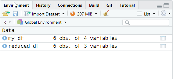
reduced_df = my_df[, -4]

Running the code above will create a new object called reduced_df in the Environment. As we can see, it consists of 6 observations of 3 variables as compared to the original data frames 6 observations of 4 variables (which makes perfect sense since we asked R to remove one variable.

Fig 1. Defining part of a data frame as a new object

Here is what the new data frame looks like in the console:

  ID age gender
1  1  40      m
2  2  51      f
3  3  32     nb
4  4  23      f
5  5  55      f
6  6  68      m

Overwriting elements of an object

Let’s now have a look at the second case, in which we use part of an R object as the left-hand-side argument of object definition. As mentioned above, this corresponds to overwriting the existing values of those elements with new values. If we want to overwrite elements of an object, we must consider two rules:

First, the new values must conform with the type of the object. We should overwrite numeric value only with numeric value, character strings with only with other character strings, and so on. If we overwrite existing values with values of different types, R will not return an error message. Instead, it will coerce the object such that all elements are of equal type. For example, trying to overwrite elements of a numeric or Boolean object with a character string will turn the whole object into a character string. If we overwrite an element of a numeric vector with a Boolean value (TRUE or FALSE), the object will remain numeric, and the new values will be interpreted as either 1 or 0, and so on.

In case of a data frame, each column works as its own object, that is, messing up one variable in this way will usually not mess up the other variables.

However, if we overwrite a complete row of the data frame, we can potentially mess up the whole data frame, because now we tamper with elements of each column.

Second, we need to tell R the correct number of new values for the elements we want to overwrite. For example, if we want to overwrite two elements of a vector, we need to define the new values in a vector of length two, and if we want to overwrite the elements of a \(3\times2\) matrix, the new values must be defined either in a \(3\times2\) matrix or as a vector of length 6 (in the latter case, R will simply overwrite the old values with the values contained in the vector by filling columns from top to bottom and then moving to the next column). There is an exception to the second rule: we can always specify a single value as the new value. In this case, R will overwrite all of the old values with this new value.

Let’s look at a few examples using the original data frame we defined above.

# The first participant entered the wrong age; we need to overwrite it with the correct value
my_df$age[1] = 41

# We want to capitalise the letters in our gender variable; overwrite the 3rd column (option A)
my_df[,3] = c('M', 'F', 'NB', 'F', 'F', 'M')

# overwrite the 3rd column (option B)
my_df$gender = c('M', 'F', 'NB', 'F', 'F', 'M')

# Participant 6 wants to retract their data we need to overwrite the 6th row with NAs
my_df[6,] = NA

Here is what the data frame looks like after we have redefined the values as per the code above:

  ID age gender employment
1  1  41      M       TRUE
2  2  51      F       TRUE
3  3  32     NB       TRUE
4  4  23      F       TRUE
5  5  55      F       TRUE
6 NA  NA   <NA>         NA

Note that R has a slightly different way of showing that a value is NA (not available, i.e., missing) in the console whenever the object type is a character string. Rather than simply showing NA as it does when objects are numeric or Boolean, R will instead show for character strings. This is purely cosmetic, that is, it has no consequences for the way we write code or how R evaluates it.

If we inspect the object using RStudio’s viewer, instead, all NA values will be shown as NA irrespective of their type.

Using numerical indexing to overwrite variable names

Remember the names() function we used previously to assign new names to the variables in a data frame? This function allows us to obtain the current variable names of a data frame. If we call it and feed it the name of a data frame as its function argument, R will return of character vector containing the names of all column contained in the data frame.

The names() function also allows us to overwrite the existing variables names if we redefine the object returned by the function call as a character vector of equal length (i.e., one element per column of the data frame). Back then we noticed that using the names() function might become tedious if a data frame contained a lot of variables. However, by using numerical indexing, we can circumvent the need to explicitly rename each variable in a data frame.

Since the names() function returns a character vector, we can use numerical indexing to pinpoint the variable names we are interested in. For example, we could ask R to tell us the name of the 2nd variable of a data frame or to overwrite the name of the 4th variable. Here is what the code would look like (we will be using the data frame we worked with above):

# obtain the name of the data frame's 2nd variable
names(my_df)[2]

# assign a new name to the 4th variable ('employed' instead of 'employment')
names(my_df)[4] = 'employed'

Running the code above prompts R to return the name of the data frame’s 2nd variable in the console:

[1] "age"

This is what the data frame looks like after renaming the 4th column.

  ID age gender employed
1  1  41      M     TRUE
2  2  51      F     TRUE
3  3  32     NB     TRUE
4  4  23      F     TRUE
5  5  55      F     TRUE
6 NA  NA   <NA>       NA

Technically, we must place the brackets used for indexing directly after the closing parentheses of the function call. Placing the brackets inside the parentheses instead resulted in error messages in previous versions of R. However, in the more recent versions of R, placing the brackets behind the name of the data frame inside the parentheses of the function call will also work. in other words, the two following lines of code produce identical results:

# obtain the names of the first three variables
names(my_df)[1:3]

# alternative code that yields the same result
names(my_df[1:3])